Inter-Egg Correlation
An alternative to the prediction-based analysis of the EGG data is based on the reasonable assumption that if an effect results in deviations at a specified time, there should be some non-zero level of correlation between the eggs at that time.
A general procedure for determining whether there is any effect on the Eggs from global events, even those which are unknown or insufficiently newsworthy to provoke a GCP prediction, is to examine the intercorrelations across the eggs. Given that they are independent sources of data, and widely dispersed so that no ordinary local perturbative forces could simultaneously and similiarly affect them, there should be no tendency for the correlation matrix to show anything but chance fluctuations. On the other hand, if we see a tendency for correlation among the meanshifts or the corresponding Chisquare values generated by the individual eggs, this indicates a global source of anomalous effect in accordance with the GCP’s general hypothesis.
An early attempt was made to explore this possibility looking at a single day’s data. Although this effort appeared promising, the correlational approach needs the power of large amounts of data to mitigate the extremely small hypothesized effect. Doug Mast has developed an analytical approach and software that is capable of assessing the intercorrelations among the eggs across months and years of data. In earlier work using these procedures, there were interesting results, but some concern about possible non-independence of multiple measures. This approach, documented as Version 1, looked at the counts of correlations at various levels of significance, and showed promise of identifying significant intercorrelation. It led Doug to further creative effort to establish a fully robust analysis. He says:
My investigation of inter-egg correlations has continued, using a large number of controls and a refined method. The results seem to show significantly anomalous correlations for data from the year 1999, but not for data from the year 2000. A summary of the methods and results follows below.
The purpose of this study was to investigate whether the egg outputs show coherence greater than would be expected by chance. As in the previous preliminary study, 60-second, 60-sample signals
from individual eggs were cross-correlated with one another. For each minute of 1999 and 2000, all possible pairs of eggs with complete data were cross-correlated and Pearson correlation coefficients (r) were computed. Control data was obtained by computing correlations for randomly offset egg signals rather than synchronous signals.
For example, suppose that only four eggs (A, B, C, and D) recorded complete data for the minute starting at midnight on a given day. For that minute, the correlations recorded would be between 60-sample signals from the egg pairs [A,B], [A,C], [A,D], [B,C], [B,D], and [C,D], each recorded for the minute starting at midnight. If some global influence acted on all four eggs during that minute, the signals recorded by the eggs might presumably be correlated with one another. This procedure is then repeated for the remaining 1439 minutes of the day.
For a control case, instead of cross-correlating synchronous signals, the signal from each egg would be taken from a random time during January 1 (perhaps the minute starting at t_A = 13:41:03 for egg A, the minute starting at t_B = 03:12:28 for egg B, etc.). Then, the control correlations would be between the offset pairs [A(t_A),B(t_B)], [A(t_A),C(t_C)], [A(t_A),D(t_D)], [B(t_B),C(t_C)], [B(t_B),D(t_D)] and [C(t_C),D(t_D)]. For each day, control runs were done for 1440 sets of temporal offsets. This procedure helps to ensure that any statistical artifacts appearing in the synchronous correlations will also appear in the control correlations.
The previous preliminary analysis employed a thresholding procedure, based on the idea that 10% of the correlations should have r values above the threshold corresponding to p=0.1. Preliminary data, and previous experience from the PEAR group with random event generators, suggested that correlation anomalies are more likely to appear as small, frequent deviations from chance expectation than as large, rare deviations. For this reason, the previous thresholding procedure was modified to use a single, lower threshold, such that |r| would be expected to be greater than the threshold r0 exactly half the time. For each cross-correlation, a hit
was recorded for |r|>=r0 and a miss
for |r| < r0; theoretically, the number of hits and misses should be exactly equal, and the probability of obtaining a given number of hits can be easily computed. For 1999, the number of hits
of this kind was much larger than expected by chance.
In addition, moments of the correlation coefficient r were also recorded using sums of r, |r|, r^2, r^3, |r|^3, and |r|^4. For each of these sums, the probability density function (PDF) is easily computed using the analytically known PDF of r and the central limit theorem. Analysis of the data for 1999 suggested that the sums of r and r^3 were no larger than expected by chance. However, the sum of |r| was much larger than expected for 1999. Sums of r^2, |r|^3, and r^4 were also larger than expected, but graphical display of accumulating z-scores clearly indicated that the curves were not independent.
The same analysis was carried out for the year 2000. Based on the 1999 results, the hypothesis to be tested was that the number of above-threshold hits, and the sum of |r|, would be larger than expected by chance. This hypothesis was not confirmed, although the results are interesting.
The numerical results can be summarized as follows. Each result is shown as a z-score and single-tailed p-value in the format z (p).
Values computed using the analytical PDFs are shown in the first column. The second column shows values computed using empirical Gaussian PDFs based on the mean and variance of the 300 controls for each year. The number of synchronous cross-correlations was N=75833818 for 1999 and N=197478113 for 2000. (The increase in N is due to the growth of the egg network.)
      N (|r|>r0) [analytic PDF]   N (|r|>r0) [control PDF]

    1999 2.549 (.00540)    2.577 (0.00499)
    2000 1.106 (.134)      1.154 (0.124)

      Sum of |r| [analytic PDF]  Sum of |r| [control PDF]

    1999 2.613 (0.00448)    2.648 (0.00405)
    2000 0.784 (0.216)      1.172 (0.121)
Clearly, the data for 2000 do not show the same phenomenon found in that of 1999. If the effect size [z/sqrt(N)] were constant, all the entries for 2000 would have astronomically small p-values, since N was much larger. So it appears that either any real effect for 1999 didn’t occur in 2000, or else the intriguing results for 1999 were a fluke abetted by my semi post-hoc analysis (i.e., I designed the refined method after gaining some experience with the 1999 data). I don’t know what to conclude, except for a big hmmmmmmmmmm,
which I guess is often the case in this business.
I responded with a suggestion for a comprehensive look, computing an additional row for the table using an unweighted Stouffer Z to combine the two years’ data for an overall look at the question. This yields a result that remains significant at the two-sigma level:
        N (|r|>r0) [analytic PDF]    N (|r|>r0) [control PDF]

     Stouffer Z
     1999 & 2000  2.584 (0.00488)    2.638 (0.00417)

          Sum of |r| [analytic PDF]  Sum of |r| [control PDF]

     Stouffer Z
     1999 & 2000  2.402 (0.00815)    2.701 (0.00346)
From this perspective, which is one way to look at replication of subtle phenomena, the case for an intercorrelation of synchronized eggs is pretty good, with probability on the order of a few parts in a thousand.
Doug responded with a more robust calculation:
To combine the two years for an overall result seems natural. I think it’s better, though, to do the full analysis for both years’ data (i.e., directly compute N(|r|>r0) and Sum(|r|) for the full two-year data set, and analyze using the appropriate analytic and control PDF’s for the larger N). The results are given below on the lines1999 & 2000 (TDM).
            N (|r|>r0) [analytic PDF]   N (|r|>r0) [control PDF]

    Stouffer Z        2.584 (0.00488)     2.638 (0.00417)

    1999 & 2000 (TDM)   2.283 (.0112)     2.271 (0.0116)

            Sum of |r| [analytic PDF]  Sum of |r| [control PDF]

    Stouffer Z        2.402 (0.00815)     2.701 (0.00346)

    1999 & 2000 (TDM)  2.043 (0.0205)     2.271 (0.0116)
The numbers from the comprehensive calculation in the last line above should be considered more accurate than the Stouffer-Z numbers. They still show an arguably significant effect, though not as significant as the calculations for 1999 alone. Of course, the effect size for the full data set is much smaller than that indicated by the 1999 data alone. The question may be asked whether the results for 1999 are scientifically valid evidence, given that the tests were designed based on the experience of the previous investigations. In this context, our discussion of statistical designs and procedures has continued, and addresses in depth certain issues such as the definition of a proper test
of the explicit and implicit hypotheses. This
technical discussion will be of interest to anyone who is concerned with the viability of the evidence for inter-egg correlations.
Graphical Representations
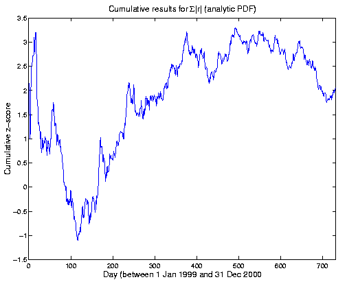
The results for the two years can be visualized graphically. In the following figure, the running or cumulative mean of the Z-scores for each day is shown as it develops over time. Plotted on the y-axis are Z-scores for the sums of |r| up to each day on the x-axis. That is, if there were N_day total trials from 1 Jan 1999 through the current day, the value plotted would be
         ( Sum[|r|] from 1 to N_day ) - mu(N_day)
    Z(day) =  -------------------------------
                        sigma(N_day)
where mu and sigma are the theoretical mean and standard deviation of Sum(|r|) for N_day trials. The expectation value of Z is zero; a constant effect size would yield a curve going as sqrt(N); and a constant p-value would be a horizontal line (I think). The end point is the overall Z score (Z for N_day -> N_final).

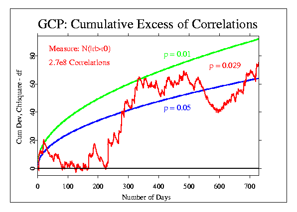
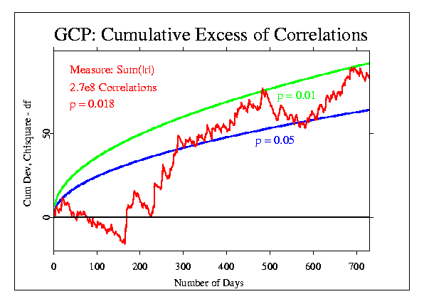
These data can be displayed in a number of different ways, of course. For most of the event-based analyses, we use a format that accumulates the deviations from expectation across seconds, minutes, or other blocks of data. This is done by converting the mean of the block of data to a Z-score ((Mean - Mu)/Sigma), where Mu is the expected mean and Sigma is the standard error for the mean. The resulting Z is squared, to give a positive, Chisquare-distributed quantity, with one degree fo freedom (df). The Chisquares are additive, and a composite Chisquare for an event or a series of events is obtained by summing them. Graphically, we can display the progressive accumulation of evidence by drawing the cumulative sum of (Chisquare - df), which has the form of a random walk around expectation zero (plotted here as a horizontal line) if there is no consistent deviation. If there is an effect, however, the random walk will have a trend away from the expectation line.
The following figures show the correlation data treated in this way. Doug provided the data for each day of the two years, in the form of the total number of correlations, the number of cases where the absolute value of the correlation was greater than expected (N(|r|>r0)), and the sum of the absolute value of the correlations for each day (Sum(|r|)).


